State Estimation: Kalman Filter Tutorial (Part 3)

This is the 3rd (and final) part of a tutorial about the Kalman Filter for state estimation. Why do we care about state estimation? State Estimation uses math to do what the brain does automatically: combine noisy sensors into a “best guess” estimate. This lets us observe all kinds of systems that can be defined mathematically.

Part 1 discusses the high-level background on State Estimation and how to create system and measurement models.

Part 2 introduces the Extended Kalman Filter equations needed in order to estimate the state of a robot lawnmower.

Finally, this tutorial discusses implementing the EKF for a differential drive mobile robot (ie., a robot lawnmower!), including pseudocode. Our EKF includes: 1) System Update and 2) GPS Measurement Update. Quick disclaimer on my pseudocode… I wrote this using MATLAB syntax. But I havent tested it, so take it as a “guide.”

Implementing System Update

We’re about to implement the Extended Kalman Filter system update for a mobile robot. Here are the relevant EKF system update equations. For a conceptual discussion on the update equations, refer to KF Tutotial Part 1. As a reminder,  represents the best estimate of the state vector while  represents the covariance (or uncertainty) in that estimate.

And remember that our differential drive mobile robot uses the state: . The differential-drive transition equation as we have derived it, in the system update, is expressed using the following equations:

Also, the matrix is the Jacobian of the system update function:

Now lets write some code for the system update, following Matlab notation.

function [state_pre, P_pre] = system_update(state, P, Qk, dt)
% state = [x, y, tht, v, omega]'

% Update State: x_pre = f(x,u), where x=state and u=0
state_pre = [state(1) + state(4)*dt*cos(state(3));
             state(2) + state(4)*dt*sin(state(3));
             state(3) + state(5)*dt;
             state(4);
             state(5);

% Calculate Fk
Fk = [ 1 0 -state(4)*dt*sin(state(3)) dt*cos(state(3)) 0;
       0 1  state(4)*dt*cos(state(3)) dt*sin(state(3)) 0;
       0 0          1                      0          dt;
       0 0          0                      1           0;
       0 0          0                      0           1];

% Update Covariance: P_pre = F*P*F' + Qk
P_pre = Fk*P*Fk' + Qk

It’s also worth mentioning that is the “system noise” covariance matrix, which is more or less a tuning parameter. The  diagonal elements represent state variance during a single system update.

Implementing GPS Measurement Update

The GPS measurement with a lever arm offset can be expressed as:

Which is what we will use for the GPS measurement update. Here are the EKF Measurement Update equations:

Where , and is the covariance matrix for the GPS measurement. In this case, .

Lets do the code for the measurement update!

function [state_post, P_post] = meas_update_gps(state, P, z, Rk, dt, off)
% state = [x, y, theta, v, omega]'
% off = [x_off, y_off]' <- this is the lever arm offset
% z = [x_gps, y_gps] <- this is the actual GPS measurement reading

% Calculate Hk
Hk = [ 1 0 -off(1)*sin(state(3))-off(2)*cos(state(3)) 0 0;
       0 1  off(1)*cos(state(3))-off(2)*sin(state(3)) 0 0];

% Find the expected measurement: h(state)
gps_est = [state(1) + off(1)*cos(state(3)) - off(2)*sin(state(3));
           state(2) + off(1)*sin(state(3)) + off(2)*cos(state(3))];

% Find Kalman Gain
K = P*H'*(H*P*H'+Rk)^-1;

% Find new state:
state_post = state + K*(z-gps_est);

% Find new covariance:
P_post = P - K*Hk*P

Putting it All Together

Now lets pull our two functions together to come up with our Extended Kalman Filter.

function [state, P] = extended_kalman_filter(state, P, z_gps)
% state = [x, y, theta, v, omega]'
% P = covariance matrix
% z_gps = [x_gps, y_gps] 
% Goal: Use the new GPS measurement to update the EKF state and covariance

% Set constants (Or pass into the function)
dt = 0.1;          % 10 Hz
Q = diag([0.01, 0.01, 0.001, 0.3, 0.3]);
Qk = Qk(dt); % <- System (Process) Noise
R_gps = [0.1^2   0; 
      0    0.1^2];
Rk_gps = R_gps*dt; % <- Measurement Noise
off = [0.25; 0];  % <- GPS lever arm offset. x_off = 0.25, y_off = 0

% Extended Kalman Filter:
[state_pre, P_pre] = system_update(state, P, Qk, dt);
[state, P] = meas_update_gps(state_pre, P_pre, z, Rk, Rk, dt, off);

We now have a functional extended kalman filter that can be placed inside a loop to estimate the robot state using GPS measurements.

A neat fact: All five states will be observable! It’s true- using GPS measurements plus knowledge of the robot system, it is possible to extract a best guess for position, heading, velocity, and angular velocity of the robot. This same approach can be applied to any other system that can be modeled with differentiable equations… simply replace the EKF equations with the equations for the new system, and you are in business (also make sure your system is Observable- but that’s a discussion for another day).

A couple easy ways to improve our mobile robot Extended Kalman Filter:

1. Add new measurements. Everyone wants more measurements! Another typical mobile robot measurement is “wheel odometry” which essentially observes the wheel rotation using incremental sensors attached to the robot. This provides a huge improvement because you can get odometry readings at, say 50 Hz whereas GPS is typically slower.
2. Improve the system. Note that the measurement system always uses an old heading to propagate the state. It has been shown that a more precise approach is to use the angular velocity to propagate this heading to the “midpoint” of each measurement. This, naturally, results in a far more complicated system update- But it has significantly better results (maybe an order of magnitude better, depending on how large the timestep dt is).

And of course, the same Extended Kalman Filter procedure applies to many other situations (surprisingly, autonomous robot lawnmowers are not the only use for the EKF). In fact, EKFs are a go-to approach for most state estimation problems in existence today… How do rockets determine their orientation while trying to land? I would take any bet the rocket uses an EKF or EKF-related algorithm. Enjoy the newfound power of state estimation! Thanks for reading.

State Estimation: Kalman Filter Tutorial (Part 2)

State Estimation uses math to do what the brain does automatically: combine noisy sensors into a “best guess” estimate. Part 2 of this tutorial dives deeper into the math behind state estimation. In particular, I discuss the “optimal” combination of all data using the Extended Kalman Filter. First, we’ll review the scenario. Second, we’ll go over the EKF on a conceptual level, then move forward on to the math. As always, the goal here is to implement something at the end of the tutorial! In this case, we should be able to program an optimal state observer.

Make sure to visit Part 1 to learn the high-level background on State Estimation and how to create your system and measurement models for the system of interest.

Scenario Review

You are a robot lawnmower, e.g. the cartoon below.. You receive GPS data sporadically. But GPS data sucks; it is very noisy. State Estimation uses GPS to tell you where you are, where you are heading, and how fast you are moving. This is important if you want to, oh, say, drive yourself!

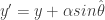
Your state is:  .  In plain English, we care about the x-position, the y-position, heading, forward velocity , and angular velocity . The forward velocity and angular velocity is taken at the mower origin (your point).

The robot lawnmower differential drive system model uses the following equations to propagate the state from timestep to timestep :

And the GPS makes a location measurement which is related to the state via the following measurement model:

Extended Kalman Filter Concept

The Extended Kalman Filter seeks to estimate the true state of a system given noisy measurements. It falls into a class of algorithms within systems engineering called a state observer, and happens to be quite popular.The Extended Kalman Filter tracks the state estimate using a “best guess” vector, , and a covariance (i.e., uncertainty) matrix, .

To visualize the EKF, imagine walking down a hallway. Your body tells you how far you move, and your eyes show you exactly where the door is at the end of the hall. Now imagine walking with your eyes closed. Your body tells you how far you move, but your eyes cannot measure the location of the door. When you take one step, you know your location fairly well. After you take ten steps, however, you might not have any solid idea besides “somewhere down this hallway.” Your brain functioning occurs in two discrete steps in this conceptual example: 1) A prediction (how your body moves), and 2) A measurement (your eyes). When your eyes cannot give you a measurement, you can still guess you location with some level of uncertainty.

The EKF operates using two steps, which should sound familiar from the past example:

1. Predict (a.k.a. System Update): The EKF propagates the state estimate from timestep to timestep using the known system model. The covariance increases.
2. Measure (a.k.a Measurement Update): The EKF applies a measurement update using the measurement model. The measurement re-aligns the state estimate with the measured values. The covariance decreases.

The EKF “magic” occurs between the covariance and the state. As the system update and measurement updates progress, the covariance robustly incorporates new measurements to generate a new best guess state estimate.

Extended Kalman Filter Math

Lets get into the heavy-duty EKF math! This can also be found on Wikipedia quite handily. The system model and measurement models, respectively, are shown:

Where and represent the nonlinear system and measurement models, respectively. The additive system noise, , and measurement noise, , are both zero mean Gaussian noise with associated covariance matrices:

Which just means the covariances are $latex \boldsymbol{Q}_k$ and $latex \boldsymbol{R}_k$, respectively.

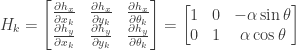
In order to use nonlinear functions and , the functions must be “linearized.” How to do this? Well, you need to take the Jacobians of and at the operating point, , during each time step. Interesting, this is the only significant math difference between the Extended Kalman Filter and Kalman Filter. These matrices are:

The typical System Update (Step 1) is performed according to the following equations:

Finally, the Measurement Update (Step 2) is applied to the EKF:

The Kalman Gain, determines how much to rely on the new measurement over the old prediction. If no measurement update is possible, then the update may be skipped by replacing the above equations with simply:

Whew! Thats a lot of math- But truly, it is nice and compact, and the EKF can in fact be written in just a few lines. So, this is about it for Part 2… While I am still aiming for an implementation, I must admit this does not quite look implementable just yet. Look out for Part 3, which will expand the EKF equations in the context of the robot lawnmower estimation problem, and ideally toss in some relevant code to demonstrate an approach to writing an EKF.

State Estimation: Kalman Filter Tutorial (Part 1)

State Estimation uses math to do what the brain does automatically: combine noisy sensors into a “best guess” estimate. In today’s world of increasingly cheap, internet-enabled hardware, state estimation allows software and hardware engineers to find the true signal out of multiple noisy sensors. A GPS and altimeter combination provides better altitude data than either sensor alone. An accelerometer fused with a gyroscope and magnetometer generates a complete 3-dimensional orientation output. Or, imagine a basketball with an embedded accelerometer and an overhead camera tracking system determines the basketball location in full 3-dimensions.

This tutorial provides a basic introduction to state estimation and begins to derive related math with an eye towards actually writing a relevant estimation program. A Kalman filter example will surface in part 2 of this series.

What is State Estimation?

First: Lets start with an example… You are a robot lawnmower. You receive GPS data sporadically. But GPS data sucks; it is very noisy. State Estimation uses GPS to tell you where you are, where you are heading, and how fast you are moving.

Another example… You are a mobile phone, which just so happens to have a nifty motion coprocessor. Maybe you want to know when someone is driving, walking, or holding you to their face. Your sensors measure acceleration, angular velocity, and a magnetic field. State Estimation gives you the best possible 3-dimensional orientation you can extract from your cheapo 2-dollar sensors.

In technical terms, state estimation extracts the best-guess internal state of a system given the system model and measurement model. But before getting too math-heavy, lets (roughly) define what is meant by a system model and measurement model:

1. System model: typically a few math equations describing the system. The system model lets you predict the state given the previous state.
2. Measurement model: a few more equations describing the measurement. The measurement model lets you update the state given sensor measurements.

The predict/update loop is the heart of state estimation, particularly all Kalman Filter variants. First, predict the next state. Second, update the prediction using measured values.

Creating the System Model and Measurement Model

The most difficult part of state estimation (and, in fact probably the most important) is creating the following three fundamentals components: 1) the state to estimate, 2) the system model, and 3) the measurement model.

Equations for the system models and measurement models must be a function of the state. On the surface, this is simply common sense- for example, to return to the lawnmower scenario, your GPS measures your position; your GPS does not measure the position of the lawnmower next to you, nor does it measure the height of the grass. However, a wise choice of state variables is one of the difficulties behind learning state estimation.

Lets begin with choosing the state. The state consists of all the parameters to be estimated. A few examples…

Lawnmower: A valid choice of state variables for a robot lawnmower is: [x position, y position, heading]. A particularly wise choice of state variables for a lawnmower (or any differential drive robot) is: [x-position, y-position, heading, forward velocity, angular velocity]. Both options are equally valid; the measurement models and system models will look slightly different to reflect the differences in state (remember the system and measurement models may be a function of the state ONLY).

Phone Orientation: A valid choice of state variables to filter orientation might look like: [3-D orientation, 3-D angular velocity]. Or the state could simply be [3-D orientation]. Either would work, but the models would look slightly different.

Let’s pursue the Lawnmower example (this is, after all, a robot lawnmower blog).

1. State: Say the state is [x-position, y-position, heading, forward velocity, angular velocity]. We’ll abbreviate the state as follows: . Where simply refers to the “vector” of state values. This is typical state estimation notation.

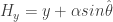
2. System Model: The system model answers the question “What happens during each timestep?” At each new timestep (the time change between successive timesteps is labeled ), a robot lawnmower moves a certain distance, which happens to be . This motion is distributed between the x and y coordinates according to the lawnmower’s heading. Therefore, we can come up with equations to move the position from timestep to timestep .

Additionally, the heading changes as a result of the angular velocity:

Finally, all we can say about the remaining states and is that we think they stay roughly the same. So our last equations are:

Which completes the robot lawnmower 2-dimensional system model.

3. Measurement Model: The measurement model answers the question “What does this sensor measure?” GPS measures the position of the lawnmower robot. When the GPS is directly over the desired state, then the measurement equations are quite simple:

No problem. Now lets imagine the GPS is offset from the estimated state by some amount , .This is where the measurement model becomes more interesting. Your GPS measurement is now a function of the heading :

Notice the additional terms constitute a rotation matrix around the true position of interest, and . This completes the robot lawnmower GPS measurement.

Conclusion, Part 1

State Estimation is a powerful field of systems and control algorithms, but is not beyond reach for a wide variety of real-world problems. To begin, derive equations for the system model and measurement model as a function of the state… The “state” describes what parameters are to be estimated. The “system model” describes the state’s natural progression over time, while the “measurement model” describes a measurement in terms of the state. A wise choice of state variables allows for simple system/measurement models.

In this tutorial, the mathematical framework for state estimation was discussed and derived for a hypothetical robot lawnmower. Part 2 will discuss parametric filters, specifically the Extended Kalman Filter, which uses the derived system and measurement models to correctly estimate the true state using noisy data.

 

“Bi-Segment” Lawnmower Antenna

Imagine a lawnmower antenna: The antenna provides a simple analog output. The lawnmower robot reads the output, interprets its velocity, and can determine exactly how far away its “edger” is from a flower bed… Which produces a beautiful trim. That would be nice.

Unfortunately, as is always the case, reality is not so nice. An antenna is a tough thing to get right. A spring-semester senior project created a hardware antenna to strap on to the front of the lawnmower. The antenna has two segments and can contact the wall at the end of either segment (see the below figure for an example image). We’ll call segment 1 the segment closest to the robot, and segment 2 is the outer segment (looking at a single antenna only). The joint between segments 1 to 2 is fixed at approximately 90 degrees. An analog potentiometer measures the rotation of the first segment.  The problem, now, is to use the analog potentiometer output to control the robot’s distance to the wall. As experimentally determined, a PID control is less-than-satisfactory for this situation. An ideal control case would be a two  -step process:

1. Use the measurement to estimate the robot’s state from the wall (distance offset and antenna offset).
2. Use the full knowledge of the robot state to control the robot’s distance and angle offset.

Naturally, step 1 leads to a  Kalman Filter. In this case, the system is nonlinear, and a typical Kalman Filter is not going to work. The question necessarily addressed first is “How nonlinear is this antenna”?? Solving for the antenna position is a piecewise problem: Given the state , what is the antenna angle measured by the sensor? Segment 1 and Segment 2 can each contact the wall in two places:

Where and are the lengths of segment 1 and the length of the hypotenuse between segments 1 and 2. These equations result in four different possible angles for the antenna. Now: The next step is to eliminate physically impossible configurations: 1) Antenna Max/Min, 2) Any antenna that passes through the wall at any point (assuming, as always here, that the wall is infinitely flat). The possibilities we are left with are valid antenna configurations. The result below shows the right antenna angle mapped as a function of the distance and heading offset from a wall. I used nominal settings, with antenna segment length of 0.4m and 0.4m each.

This sensor is apparently quite nonlinear. Notice the discontinuity where the segment contacting the wall switches from Segment 1 to Segment 2. This discontinuity helps explain why the first attempt at PID control failed- linear assumptions were simply invalid. Also scary: there are several points where a single sensor reading corresponds to multiple possible states! Typically, filtering problems involve measurements which are a linear combination of the state (ie, a “many-to-one” mapping). Our bi-segment antenna has a “many-to-one” mapping and also a “one-to-many” mapping. The red area on this chart shows the (small) section where there is a “one-to-many” mapping. I hope that this is small enough to ignore for now.

To wrap things up here, it is clear that our bi-segment antenna is a frighteningly non-linear measurement. Also, because we have a piecewise measurement function, typical Extended Kalman Filter equations (which require analytic partial derivatives) will not work here. As a preview, I believe an Unscented Kalman Filter may have some hope to filter this problem- But I’m not 100% if even that will work. To continue with this analysis, I would like to compare the sensor output readings as a function of robot state for other antenna configurations (bisegment with different antenna parameters, and circular antennas). Is there a way that we can manipulate the sensor in hardware to make the system more easily controllable?? These are the questions that simulation hopes to answer.

 

 

CWRU Cutter Hex Update/ End of Life Announcement!

As of June 2013, CWRU Cutter Hex is officially retired! On to new challenges with CWRU Cutter Se7en (or whatever the new group decides to name our next generation robot). Some background for the last six months: CWRU Cutter Hex competed in the 2013 Autonomous Snowplow competition– We placed 4 out of 10, which was the highest placement by any new team this year. Two grad students working on the robot (myself and Charles) also graduated and have moved away from the project.

Which brings me to the current plan for the robot and for this blog:

1. The robot will live on as a research platform for autonomous lawnmowers. It is yet to be determined if the robot will compete in next year’s robot snowplow competition.

2. As a part of my MS thesis, I fully developed an Extended Kalman Filter for the robot using a GPS or any other absolute positional sensor, a lever arm offset, and severe wheel slippages (as is the case with a robot snowplow). Previous posts in the fall (ie, GPS Measurement in an EKF) were just wrong at the EKF theory and system derivation for the robot. Future posts will correct the theory and show results from both simulation and actual Autonomous Snowplow Competition data. 

3. An antenna for a robot lawnmower provides a cheap-and-dirty sensor: imagine, an analog input could tell the lawnmower exactly how the robot needs to edge a flower garden! This robot antenna is a source for future research and senior projects. 

 

 

Random-Moving Lawnmower Robots

How good are lawnmower robots that move randomly inside a buried wire (Husqvarna, Friendly Robotics)?

I put together a Matlab simulation that looks at how quickly a small lawnmower robot might be able to cover a lawn that is just 10m x 10m (100 square meters). To be specific, I wanted to look at the effects of having a large blade versus a smaller blade on a robot mower, and whether there is a linear decrease in time with a larger cutting area. It makes intuitive sense that when a robot moves in straight, parallel lines, a robot with 1/2 the cutting area will take just about twice as long to mow the same area. But, how does this work when the robot is moving randomly?

I wanted to make the simulation as simple as possible… Here are my constraints/ assumptions:

1. The robot always drives in a perfectly straight line at 0.5 m/s, and does not accelerate or decelerate.
2. When the robot hits a boundary, it chooses a random angle which will direct the robot back into the cutting zone (ie, if the robot hits the bottom boundary, it will choose a new motion angle between 0 and pi).
3. The area is discretized into 0.05 m squares. The robot “cuts” the grass in a square centered at the robot’s origin (a 0.5 m blade will cut a 0.5m x 0.5 m square of grass each time step).
4. The simulation ends once the robot has cut 95% of the grass in the cutting zone.

These are reasonable simplifications because the robot now moves randomly while cutting a specified area of grass, and I am not interested in the accelerations, decelerations, turns, or whether the cutting area is a circle or a square.

For a 0.5 meter cutting area, I found the average cutting time was around 1000 seconds. For a 0.25 meter cutting area, the cutting time increased to approximately 2600 seconds. Interestingly, the cutting time more than doubles for a 1/2 size cutting area. I found a best-fit approximation for the percentage of grass left to be mowed over time for both sizes of cutting area; The percentage of grass follows an exponential decay very well. Both best-fits are plotted here:

Percentage of grass left to be mowed over time

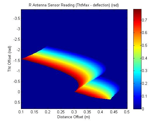
From the best-fit plot, it is clear the amount of grass left to be mowed follows an exponential decay. Specifically,  for 0.50 m, and for 0.25 m. So, a smaller cutting area takes exponentially more time than a larger cutting area for a lawnmower using random motion. I could, theoretically, create an equation to solve for the time constant based on the cutting width and desired area. To get a feel for what the random paths look like for the small and large cutting decks, see the representative paths:

Two example paths, cutting area of 0.5 and 0.25 meters.

Now, how accurate is this simulation when applied to real life?? I believe any truly random-motion complete-coverage robot will experience this exponential decay. As far as the absolute time, I cant say for sure (15 minutes for a 0.5 meter cutting area, 40 minutes for a 0.25 meter cutting area) … If the robot moves faster than 0.5 seconds on the straightaways, the time could possibly decrease from the simulation baseline; But likely, the robot will account for acceleration, decelerations, and turns, so running time will take somewhat longer.

This result makes me curious about the Husqvarna lawnmower in particular, which claims to be able to cut up to 3000 square-meters (3/4 of an acre) while the cutting width is approximately 0.25 meters. If we assume the randomly-moving lawnmower with a 0.25 meter cutting area is placed in a boundary 30 times as large, we expect the time constant on the exponential decay to be smaller by a factor of approximately 30… The exponential decay equation simplifies to show that running time scales linearly with the area of the zone to cut. So, a 0.25 meter-wide mower requires over 20 hours of operation to cut 3000 square meters!

On the other hand, if the robot can localization and drive straight paths, calculating mowing time becomes an algebra problem: For a lawnmower to intelligently cover a 10m x 10m yard with a 0.25 cutting area, it needs 40 back-and-forth lengths, 1 side-to-side length of 10 meters, and 78 total turns. At 0.5 m/s, assuming no accelerations or decelerations, total running time is 14 minutes. This will scale linearly; a 3000 square meter area will take approximately 7 hours, which is a significant improvement over 20 hours. Also, there will be an additional benefit because the random path involves considerably more turns than the intelligent path, meaning even more time is lost accelerating and decelerating. Clearly- a smart robot is the way to go!

Observability of GPS Measurements (in an Extended Kalman Filter)

Given a robot state , is it possible to use a Kalman Filter to observe the full state using only measurements from a GPS?

Near the end of my first post, Differential Drive Steering and Kalman Filter Basics, I mentioned that my very first simulation used a GPS measurement plus some unspecified heading measurement. I justified the heading measurement: “I’m worried that the orientation is currently unobservable; So, I also added a non-biased, noisy measurement of the orientation for now. I’m not sure what physical sensor this would correspond to, but hey, its a simulation.” It turns out, if I remove the orientation sensor, the Kalman filter simulation falls apart!

In this case, I am using a GPS with a lever arm offset (see the previous post: GPS Lever Arm Offset). The measurement equations are therefore:

This leads to the linearized Jacobian of the measurement matrix, which is used in the Extended Kalman Filter:

As a sanity check, the Observability of a system will show whether it is possible to recreate all states in a system using a given measurement with measurement sensitivity . For a linear, time-invariant system, the Observability check is:

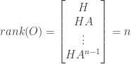
Where is the rank of the state matrix, . For our simple system, is the identity matrix…

And I dont care about because that represents the control input, which is not used in the observability derivation. Now, even though the system itself is non-linear, a Kalman filter is by nature a linear observer and I have linearized the measurement in order to use the Kalman filter equations. Therefore, the above observability test should hold using the known and matrices. It is clear that because is identity, the Observability matrix only has rank 2, which is not equal to the number of states (). So in conclusion, an Extended Kalman Filter with the state equal to and a single GPS measurement of is NOT observable.

There’s a few options at this point…

1. Add a new measurement: Maybe a magnetometer or something to get an estimate of the heading
2. Try to back out orientation based on the past states of the GPS- This would work sufficiently okay if the GPS did not have a lever arm offset
3. Expand to include velocity states
4. Use a particle filter, which I have shown already works very well with GPS lever arm offsets

I’m leaning towards including velocity states (a good idea for a Kalman filter anyway), or switching over to a particle filter (which we plan to do in the future for other sensors).

CWRU Cutter Robot Architecture: Low Level

We’ve structured the CWRU Cutter robot into various components which should be, more or less, independent of each other.

1. Our low level control system uses a National Instruments Compact RIO. The cRIO includes an FPGA, a PowerPC processor, and various modules for input/output connectivity (all programmed using NI’s LabVIEW, of course… it can be a blessing and a curse). I will talk a little bit about low level hardware and software here.
2. Higher level processing is performed on a mini-ITX form factor PC, running Ubuntu and Robot Operating System. ROS provides a well defined framework for robots which is easily scale-able for research projects and certain snowplow competitions coming up in two and a half months. High level architecture is better saved for a different post (ie, we’re still not quite sure whats going on yet).

Low Level cRIO and Breakout Board

The compact RIO is responsible for 3 major tasks, which currently work quite well:

1. Encoder input/ counting (the FPGA is used to count encoder ticks)
2. Closed loop velocity control (ensures that we can command a desired velocity and the robot with drive at that speed)
3. Safety input/output (Emergency stop chain, switch input, etc)

Finally, the cRIO needs to communicate with the high level PC, which it manages using a 57.6 kbps RS-232 connection. The PC implements Rosserial to communicate velocity commands and read encoder counts- there will be a post in the future about the trials, difficulties, and lessons learned regarding Rosserial on LabVIEW.

In addition, we have a notoriously difficult-to-use 37-pin NI 9403 module for low-level digital input and output. To simplify soldering issues and consolidate analog circuity, the solution is a custom one-off printed circuit board which we use as the “lower” low-level breakout board. I also went a bit overboard, pulling 34 out of 37 pins from the 9403 over to the breakout. The 5″ x 5″ breakout board consists of the following components:

• Digital Output Buffer (the 9403 can only source/sink like 2mA)
  

  CWRU Cutter cRIO breakout PCB in EAGLE

• Emergency Stop button and 4 other on-off switches
• PWM input from a Futaba RC receiver (straight through to the cRIO)
• PWM input from a Futaba RC receiver, which passes through some analog circuity to create a remote emergency stop function
• Battery voltage and current monitoring
• 6 other analog inputs
• Software- and hardware- controlled emergency stop chain, with Relay outputs to enable/disable drive relays

The cRIO breakout 1.0 is currently functional on the robot, but it was lacking a few necessary features- so, I included all of the required components on version 2.0, shown to the right. It has yet to be populated and placed on the robot, but it will come before competition day.

The remote control emergency stop is one of the more interesting features of the breakout board. This RC Estop consists of a rectangular pulse timer, triggered at the rising edge of the PWM, and a D-flip flop triggered at the falling edge of the PWM. If the Futaba RC PWM output is greater than 50% on, the output of the RC Estop circuity is high. This value is used as an enable input on the Emergency Stop chain; The robot physically cannot drive or mow without the RC Estop being enabled. The RC Estop timing circuit schematic is shown.

555-based PWM timer

In the end, what we have (or will have, once everything is implemented) is a reliable, flexible low level system. There are plenty of inputs and outputs, and a custom hardware implementation allows us to use an RC Estop and a redundant emergency stop chain. When we are bored and have time to spare, the obvious progression for the low-level system is to combine the breakout board with a powerful microcontroller or a FPGA/processor combination for ultimate cost-effectiveness, removing the cRIO entirely… Its good to have goals.

GPS Lever Arm Offset

For aesthetic purposes, our robot’s GPS antenna is inconveniently NOT centered at the robot’s origin (directly above the middle of the wheel base). Check out a picture here: https://cwrucutter.wordpress.com/#jp-carousel-164.

This GPS lever arm offset has given us trouble for a few years. Theoretically, the GPS location on the robot should not make a significant difference. The “H matrix” that represents the GPS measurement is shown below for a lever arm offset, assuming is the true state, is the GPS measurement:

Also, is the estimated heading. In order to correctly propagate uncertainty in our Kalman filter, this H matrix would have to be linearized using a Jacobian according to the Extended Kalman Filter equations. I dont believe we’ve ever done this correctly before, causing the covariance matrices in our EKF to be incorrect. So, I decided to apply my particle filter simulation to see if it could handle a GPS with a lever arm offset… After about 30 minutes (further evidence of the ease-of-use for Particle Filters), simulation results are qualitatively indistinguishable between GPS located directly on the origin and GPS with an offset.

To generate the GPS measurement, I simply followed the above equations and added random noise with a specified GPS standard deviation. To apply the measurement update, I created a new “gps-lever-arm-offset” measurement sampling procedure. The new sampling procedure uses a given to calculate the probability that a single particle produced the generated measurement. Resampling then narrows the particle pool to include only those particle most probable to actually be true. The figure below shows the final result of a robot driving around in a circle, using GPS on the origin (left) and GPS with a 0.4 m offset (right).

Left: GPS on origin, Right: GPS offset by 0.4m

Qualitative results appear to show that the location solution is essentially the same, given that is known. Indeed, the GPS-on-origin case is simply equivalent to . So, it appears that we should be able to easily use a particle filter to fuse the measurements from our GPS.

An additional complication worth noting is that we have tried to use the “speed over ground” measurement from the GPS in the past. This seems like a useful measurement which would provide the magnitude of the robot’s velocity over a certain timestep; however, this is somewhat more difficult with a lever arm offset. The speed over ground with a lever arm offset is no longer the speed at the origin, but rather the magnitude of the linear velocity at a certain point on the robot which is also affected by rotational velocity. It may be worth an additional investigation on how to incorporate the velocity measurement, but this has, historically, caused some issues for our robot.

Range-Only-Landmarks (using a Particle Filter)

I recently implemented a simulation showing that a particle filter can be used to track a mobile robot using only range measurements from a single landmark (plus odometry). See the end of my previous post: Basics of Particle Filters. The conceptual idea is: if you look at a range measurement at a single moment in time and attempt to solve for position, the system is underdetermined… the position can exist anywhere on a circle around the landmark. But, when the measurement is used over time with odometry data, the position can be determined.

So, if we can determine the robot’s position from a single landmark, we should be able to work backwards… And in fact, we can also determine the landmark’s location relative to the robot’s origin, again using only range measurements. In my modified particle filter, I use each particle to represent the possible location of the landmark relative to the robot. The three “motions” related to odometry readings are used as the motion model (rotate the coordinate frame, move a distance, rotate again, with added noise on each motion). The range measurements are applied by resampling the particles, as usual. The figure below shows the landmark estimates as particles superimposed on the map. Note that while the particle filter is tracking the beacons relative to the robot, the figures below use the true robot location to visualize the beacon estimate.

A single beacon is located relative to the robot using only range measurements.

In the first few seconds of the simulation, the robot has a very wide idea of the landmark location (which is initialized to a uniform density across a nominally large space). After moving some distance, the robot finds where the landmark is located, and then refines the estimate over time. In this simulation, there is definitely a correlation between how far away the robot is and how well the landmark location is known… When the robot is far away, the estimate becomes much wider.

If I can find a single beacon relative to the robot, it isnt too much harder to locate two beacons:

Two beacons are now located relative to the robot.

Again, there is a wide initialization area, yet the estimates converge for both landmarks. The final result after driving in a circle is shown:

Not a bad estimate here

Because we can locate two stationary beacons relative to the robot, we can find a very basic solution for the Simultaneous Localization and Mapping (SLAM) problem: Assume beacon 1 is the origin, let beacon 2 define the x-axis… By knowing the landmark locations in a relative coordinate frame to the robot, a coordinate shift will place the robot into a global frame where the uncertainty should be equal to the sum of the beacon 1 and beacon 2 uncertainties. I will have to see if this is “good enough” for complete coverage navigation… The verdict is still out.